Uncertainty Quantification (UQ)#

Uncertainty quantification (UQ) is an emerging field in applied mathematics that aims to quantify uncertainties in mathematical models as a result of error propagation in the modeling process. This is especially important since we use the model, i.e., the potential, to predict material properties that are not used in the training process. Thus, UQ process is especially important to assess the reliability of these out-of-sample predictions.

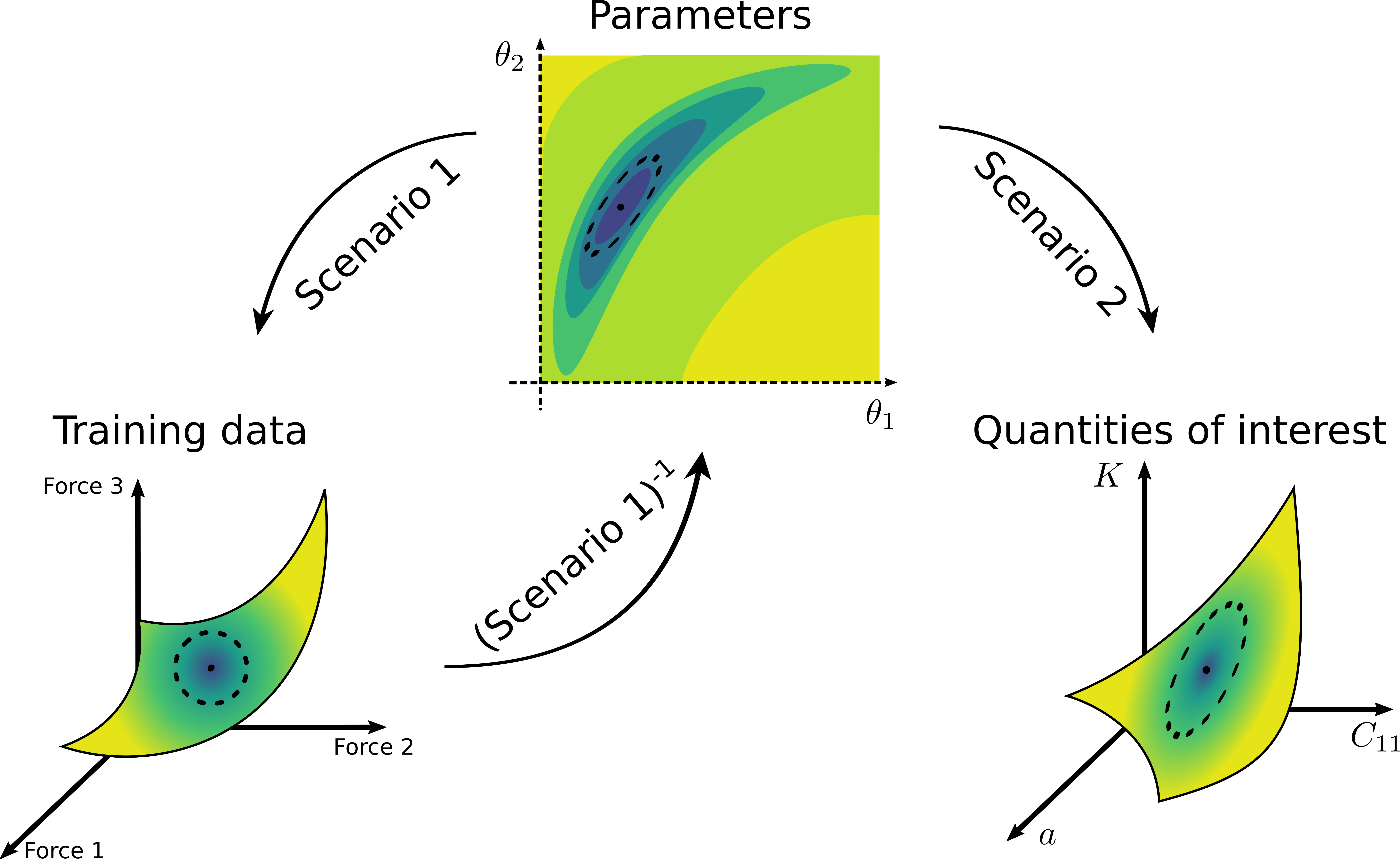
Illustration of general uncertainty quantification process. The error from the training data (represented by a dashed ellipse on the bottom left plot) is propagated to the uncertainty of the model’s parameters (the ellipse in the middle plot). Then, the uncertainty of the parameters is propagated forward further to the uncertainty of the material properties of interest (the ellipse on the bottom right plot).#

In UQ process, we first quantify the uncertainty of the model parameters (represented by the dashed ellipse on the middle plot of the figure above). Having found the parametric uncertainty, then we can propagate the uncertainty of the parameters and get the uncertainty of the material properties of interest, e.g., by evaluating the ensemble that is obtained from sampling the distribution of the parameters. As the first uncertainty propagation is more involved, KLIFF implements tools to quantify the uncertainty of the parameters.

In KLIFF, the UQ tools are implemented in uq. In the current version, there are 2 methods implemented: Bayesian MCMC sampling and bootstrapping, with the integration of other UQ methods will be added in the future.

MCMC#

The Bayesian Markov chain Monte Carlo (MCMC) is the UQ method of choice for interatomic potentials. The distribution of the parameters is given by the posterior $P(\bm \theta | \bm q)$ . By Bayes’ theorem

$P(\bm \theta | \bm q) \propto L(\bm \theta | \bm q) \times \pi(\bm \theta),$

where $L(\bm \theta | \bm q)$ is the likelihood (which encodes the information learned from the data) and $\pi(\bm \theta)$ is the prior distribution. Then, some MCMC algorithm is used to sample the posterior and the distribution of the parameters is inferred from the distribution of the resulting samples.

The likelihood function is given by

$L(\bm \theta | \bm q) \propto \exp \left( -\frac{\mathcal{L}(\bm \theta)}{T} \right).$

The inclusion of the sampling temperature $T$ is to account for model inadequacy, or bias, in the potential [Kurniawan2022]. Frederiksen et al. (2004) [Frederiksen2004] suggest estimating the bias by setting the temperature to

$T_0 = \frac{2 \mathcal{L}_0}{N},$

where $\mathcal{L}_0$ is the value of the loss function evaluated at the best fit parameters and $N$ is the number of tunable parameters.

Implementation#

For the MCMC sampling, KLIFF adopts parallel-tempered MCMC (PTMCMC) methods, via the ptemcee Python package, as a way to perform MCMC sampling with several different temperatures. Additionally, multiple parallel walkers are deployed for each sampling temperature. PTMCMC has been widely used to improve the mixing rate of the sampling. Furthermore, by sampling at several different temperatures, we can assess the effect of the size of the bias to any conclusion drawn from the samples.

We start the UQ process by instantiating MCMC,

from kliff.uq import MCMC

loss = ...  # define the loss function
sampler = MCMC(
    loss, nwalkers, logprior_fn, logprior_args, ntemps, Tmax_ratio, Tladder, **kwargs
)

As a default, MCMC inherits from ptemcee.Sampler. The arguments to instantiate the sampler are:

loss, which is a Loss instance. This is a required argument to construct the untempered likelihood function ( $T=1$ ) and to compute $T_0$ .
nwalkers specifies the number of parallel walkers to run for each sampling temperature. As a default, this quantity is set to twice the number of parameters in the model.
logprior_fn argument allows the user to specify the prior distribution $\pi(\theta)$ to use. The function should accept an array of parameter values as input and compute the logarithm of the prior distribution. Note that the prior distribution doesn’t need to be normalized. The default prior is a uniform distribution over a finite range. See the next argument on how to set the boundaries of the uniform prior.
logprior_args is a tuple that contains additional positional arguments needed by logprior_fn. If the default uniform prior is used, then the boundaries of the prior support (where $\pi(\theta) > 0$ ) need to be specified here as a $N \times 2$ array, where the first and second columns of the array contain the lower and upper bound for each parameter.
ntemps specifies the number of temperatures to simulate.
Tmax_ratio is used to set the highest temperature by $T_{\text{max}} = T_{\text{max\_ratio}} \times T_0$ . An internal function is used to construct a list of logarithmically spaced ntemps points from 1.0 to $T_{\text{max}}$ , inclusive.
Tladder allows user to specify a list of temperatures to use. This argument will overwrites ntemps and Tmax_ratio.
Other keyword arguments to be passed into ptemcee.Sampler needs to be specified in kwargs.

After the sampler is created, the MCMC run is done by calling run_mcmc().

p0 = ...  # Define the initial position of each walker
sampler.run_mcmc(p0, iterations, *args, **kwargs)

The required arguments are:

p0, which is a $K \times L \times N$ array containing the position of each walker for each temperature in parameter space, where $K$ , $L$ , and $N$ are the number of temperatures, walkers, and parameters, respectively.
iterations specifies the number of MCMC steps to take. Since the position of step $i$ in Markov chain only depends on step $(i-1)$ , it is possible to break up the MCMC run into smaller batches, with the note that the initial positions of the current run needs to be set to the last positions of the previous run.

Parallelization#

In principle, parallelization for the MCMC run can be done in 2 places: in the likelihood (or loss function) evaluation for each parameter set (see Run in parallel mode) and in the likelihood evaluation across different walkers. In the current implementation we supports OpenMP-style parallelization in the loss evaluation and both OpenMP and MPI for the sampling for different walkers when running MCMC sampling.

In general, parallelization in the sampling process is done by declaring a pool and setting it to sampler.pool prior to running MCMC, for example:

from multiprocessing import Pool

sampler.pool = Pool(nprocs)  # nprocs is the number of parallel processes to use
sampler.run_mcmc(p0, iterations, *args, **kwargs)

To do parallelization with MPI, we can utilize MPIPool from schwimmbad:

from schwimmbad import MPIPool

sampler.pool = MPIPool()
sampler.run_mcmc(p0, iterations, *args, **kwargs)

and run the Python script with mpiexec bash command.

If enough compute resources are available, we can also employ a hybrid parallelization, for example, using multiprocessing in the loss evaluation (by specifying the argument nprocs > 1) and MPI in the likelihood evaluation across different walkers. Then, we can run the Python script as follows.

$ export MPIEXEC_OPTIONS="--bind-to core --map-by slot:PE=<num_openmp_processes> port-bindings"
$ mpiexec -np <num_mpi_workers> ${MPIEXEC_OPTIONS} python script.py

MCMC analysis#

The chains from the MCMC simulation need to be processed. In a nutshell, the steps to take are

Estimate the burn-in time and discard it from the beginning of the chain,
Estimate the autocorrelation length, $\tau$ , and only take every $\tau$ step from the remaining chain,
Assess convergence of the samples, i.e., the remaining chain after the two steps above.

Burn-in time#

First, we need to discard the first few iterations at the beginning of each chain as a burn-in time. This is similar to the equilibration time in a molecular dynamics simulation before the measurement. This action also ensures that the result is independent of the initial positions of the walkers.

KLIFF provides a function to estimate the burn-in time, based on the Marginal Standard Error Rule (MSER). This can calculation can be done using the function mser(). However, note that this calculation needs to be performed for each temperature, walker, and parameter dimension separately.

Autocorrelation length#

In the Markov chain, the position at step $i$ is not independent of the previous step. However, after several iterations (denote this number by $\tau$ , which is the autocorrelation length), the walker will “forget” where it started, i.e., the position at step $i$ is independent from step $(i + \tau)$ . Thus, we need to only keep every $\tau \text{-th}$ step to obtain the independent, uncorrelated samples.

The estimation of the autocorrelation length in KLIFF is done via the function autocorr(), which wraps over emcee.autocorr.integrated_time. This calculation needs to be done for each temperature independently. The required input argument is a $L \times \tilde{M} \times N$ array, where $L$ and $N$ are the number of walkers and parameters, respectively, and $\tilde{M}$ is the remaining number of iterations after discarding the burn-in time.

Convergence#

Finally, after a sufficient number of iterations, the distribution of the MCMC samples will converge to the posterior. For multi-chain MCMC simulation, the convergence can be assessed by calculating the multivariate potential scale reduction factor, denoted by $\hat{R}^p$ . This quantity compares the variance between and within independent chains. The value of $\hat{R}^p$ declines to 1 as the number of iterations goes to infinity, with a common threshold is about 1.1.

In KLIFF, the function rhat() computes $\hat{R}^p$ for one temperature. The required input argument is a $L \times \tilde{M}^* \times N$ array of independent samples ( $\tilde{M}^*$ is the number of independent samples in each walker). When the resulting $\hat{R}^p$ values are larger than the threshold (e.g., 1.1), then the MCMC simulation should be continued until this criterion is satisfied.

Note

Some sampling temperatures might converge at slower rates compared to others. So, user can terminate the MCMC simulation as long as the samples at the target temperatures, e.g., $T_0$ , have converged.

Bootstrap#

In general, the training dataset contains some random noise. When the data collection process is repeated, we will not get the exact same values, but instead, we will get (slightly) different values, where the deviation comes from the random noise. If we train the model to fit different realizations of the training dataset, we will get a distribution of the parameters. The uncertainty of the parameters from this distribution gives how the error in the training data is propagated to the uncertainty of the parameters. However, oftentimes we don’t have the luxury to repeat the data collection. A suggestion, in this case, is to generate artificial datasets and train the model to fit these artificial datasets.

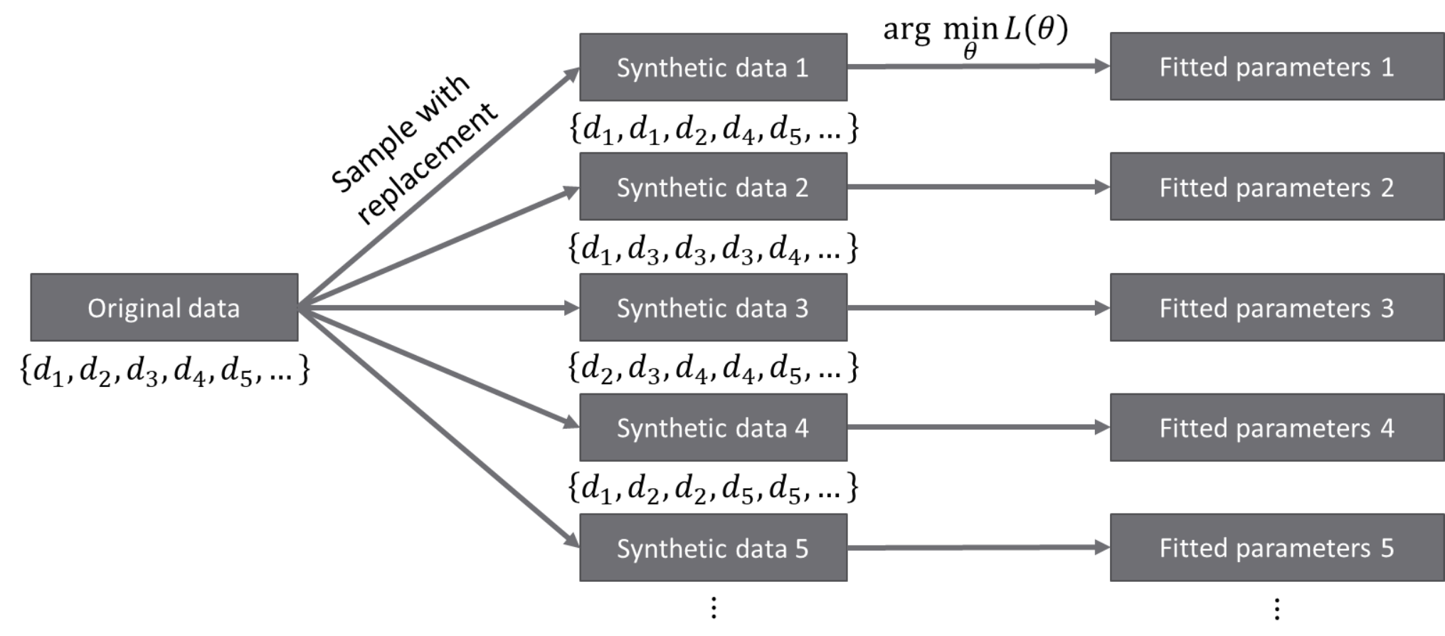
Bootstrapping is a way to generate artificial datasets. We assume that the original dataset contains $N$ independent and identically distributed (iid) data points. An artificial, bootstrap dataset is generated by sample $M$ points from the original dataset with replacement. Note that this means that there are some data points that are repeated, while some other data points are not sampled, thus the bootstrap dataset is not the same as the original dataset. The difference between the datasets gives a sense of probability in data.

Note

Although usually $M$ is set to be the same as $N$ , in principle it doesn’t need to be.

Implementation#

Bootstrapping is implemented in Bootstrap. A general workflow for this calculation is

Instantiate Bootstrap class instance.

This process is straightforward. The only required argument is the Loss instance.
```
from kliff.uq import Bootstrap

loss = ...  # define the loss function
# Train the potential
min_kwargs = ...  # Optimizer setting
loss.minimize(**min_kwargs)

bs = Bootstrap(loss, *args, **kwargs)
```
When instantiating the parent class Bootstrap, it will return either an instance of BootstrapEmpiricalModel or BootstrapNeuralNetworkModel, depending on whether we have a physics-based (empirical) model or a neural network model, respectively. When a neural network model is used, the user can specify an additional argument orig_state_filename, which specified the name and path of the file to use to export the initial state of the model prior to running bootstrap. This is to reset the state of the model at the end of performing bootstrap UQ.
Generate bootstrap datasets.

In this implementation, we assume that the training dataset consists of many atomic configurations and the corresponding quantities. Note that the quantities corresponding to a single atomic configuration are not independent of each other. Thus, the resampling process to generate a bootstrap dataset should not be done at the data point level. Instead, we should generate a bootstrap dataset by resampling the atomic configurations.

The built-in bootstrap dataset generator function was set up to perform this type of resampling. Note that atomic configurations here are referred to as compute arguments, which also contain the type of data and weights to use.
```
nsamples = ...  # Number of samples to generate
bs.generate_bootstrap_compute_arguments(nsamples)
```
When an empirical model with multiple calculators is used, the resampling is done to the combined list of the compute arguments across all calculators. Then, an internal function will automatically assign back the bootstrap compute arguments to their respective calculators. This means that the number of compute arguments in each calculator when we do bootstrapping is more likely to be different than the original number of compute arguments per calculator, although the total number of compute arguments is still the same.

Also, note that the built-in bootstrap compute arguments generator assumes that the configurations are independent of each other. In the case where this is not satisfied, then a more sophisticated resampling method should be used. This can be done by defining a custom bootstrap compute arguments generator function. The only required argument for this function is the requested number of samples.
Run the optimization for each bootstrap dataset.

After a set of bootstrap compute arguments is generated, then we need to iterate over each of them, and train the potential to fit each bootstrap dataset.
```
bs.run(min_kwargs=min_kwargs)
```
There are 2 arguments that are the same to run the optimization stage of bootstrapping, regardless if we use an empirical or neural network model. These arguments are:
- min_kwargs, which is a dictionary containing the keyword arguments that will be passed into the optimizer. This argument can be thought of as the optimizer setting.
  
  Note
  
  Since the mapping from the bootstrap dataset to the inferred parameters contains optimization, then it is recommended to use the same optimizer setting when we iterate over each bootstrap compute argument and train the potential. Additionally, the optimizer setting should also be the same as the setting used in the initial training, when we use the original set of compute arguments to train the potential.
- callback, which is an option to specify a function that will be called in each iteration. This can be used as a debugging tool or to monitor convergence.
For other additional arguments, please refer to the respective function documentation, i.e., run() for an empirical model or run() for neural network model.